The Complex-Step Trick

Ilia Kuk

October 7, 2026

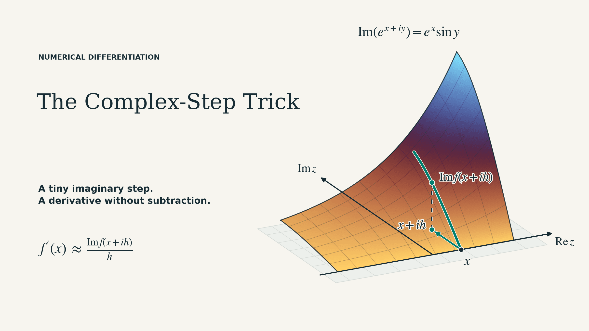
Ask a computer for the derivative of $e^x$ at $x=1$ . Give it the familiar finite-difference formula and a very small step, say $h=10^{-30}$ . In ordinary double precision, the answer is zero.

Now make that same step imaginary. The answer becomes $2.718281828459045$ , matching the usual double-precision value of $e$ .

You can try it with a few lines of Python:

import cmath
import math
 
x = 1.0
h = 1e-30
 
finite_difference = (math.exp(x + h) - math.exp(x)) / h
complex_step = cmath.exp(x + 1j * h).imag / h
 
print(finite_difference)  # 0.0
print(complex_step)       # 2.718281828459045

This is complex-step differentiation. For a suitable function, a single evaluation at $x+ih$ carries the derivative in its imaginary part. That small change can recover digits that a real finite difference has already lost.

The same idea can work when the function is an entire simulation: perturb a parameter, run the calculation, and extract the imaginary part of the output. The interesting questions are why such a tiny step survives, and what can erase it along the way.

Why a smaller step isn’t always better

The familiar starting point is

f'(x) \approx \frac{f(x+h)-f(x)}{h}.

For a smooth function, a smaller $h$ reduces the error from approximating the derivative by a finite step. But the computer also rounds its calculations. Eventually, the difference we want becomes comparable to the rounding errors in the two function values.

In the opening example, the failure happens even earlier: adding $10^{-30}$ to $1$ produces exactly $1$ in double precision. Both function evaluations receive the same input, so their difference is zero.

Using a central difference improves the approximation:

D_c(h)=\frac{f(x+h)-f(x-h)}{2h}.

Its truncation error is proportional to $h^2$ , compared with $h$ for the forward difference. Yet it still subtracts nearly equal function values. A useful model for its total error is

\operatorname{error}(h) \approx C_1h^2+C_2\frac{\varepsilon_{\rm mach}}{h},

where $\varepsilon_{\rm mach}$ measures floating-point precision and the constants depend on the function and its scale. Decreasing $h$ reduces the first term while increasing the second. This is why finite-difference error curves often have a valley: there is a useful range of steps, followed by a region where taking smaller steps makes things worse.

A derivative estimate that changes wildly when you reduce the step may be running out of numerical precision. Smaller steps do not guarantee a better answer.

Put the step in the imaginary direction

Suppose $f$ is real-valued for real inputs and has an analytic extension near the point of interest, so we can expand it in a complex Taylor series:

f(x+ih) =f(x)+ihf'(x)-\frac{h^2}{2}f''(x) -i\frac{h^3}{6}f'''(x)+\cdots.

The even powers contribute to the real part; the odd powers contribute to the imaginary part. Taking the imaginary part and dividing by $h$ gives

\frac{\operatorname{Im}f(x+ih)}{h} =f'(x)-\frac{h^2}{6}f'''(x)+\mathcal{O}(h^4).

There is our derivative estimate:

\boxed{f'(x)\approx\frac{\operatorname{Im}f(x+ih)}{h}.}

Like the central difference, it is second-order accurate. Its numerical advantage comes from extracting a component of one function value, avoiding the subtraction between neighboring evaluations.

Complex arithmetic stores the real and imaginary components separately. In $1+i10^{-30}$ , the tiny perturbation occupies the imaginary component, where it does not have to compete with the real number $1$ for significant digits. A compatible implementation can carry that perturbation through the calculation and return an imaginary part approximately equal to $hf'(x)$ .

Complex step still has truncation error. Its advantage is that you can often make that error negligible with a tiny step, without triggering the usual finite-difference cancellation.

For many well-behaved calculations, a step such as $10^{-30}$ works in double precision. It is not a universal prescription: underflow, internal numerical errors, and the scale of the problem still matter. The code evaluating $f$ must preserve the small imaginary response accurately.

Watch the error curves

For a less trivial test, consider

f(x)=e^{\sin x}+0.1\cos(7x).

We can check every numerical estimate against its exact derivative,

f'(x)=e^{\sin x}\cos x-0.7\sin(7x),

evaluated at $x_0=0.5$ . The relative error is

\frac{|D-f'(x_0)|}{|f'(x_0)|},

where $D$ is the numerical estimate.

The comparison includes forward and central differences, complex step, and two ways to improve the real finite-difference approximation. A fourth-order central stencil uses four function evaluations:

D_4(h)=\frac{-f(x+2h)+8f(x+h)-8f(x-h)+f(x-2h)}{12h}.

Richardson extrapolation instead combines central differences at two step sizes:

D_R(h)=\frac{4D_c(h/2)-D_c(h)}{3}.

For sufficiently smooth functions, both cancel the leading second-order truncation error. They can therefore reach high accuracy with larger steps. Both also retain subtraction between nearby function values.

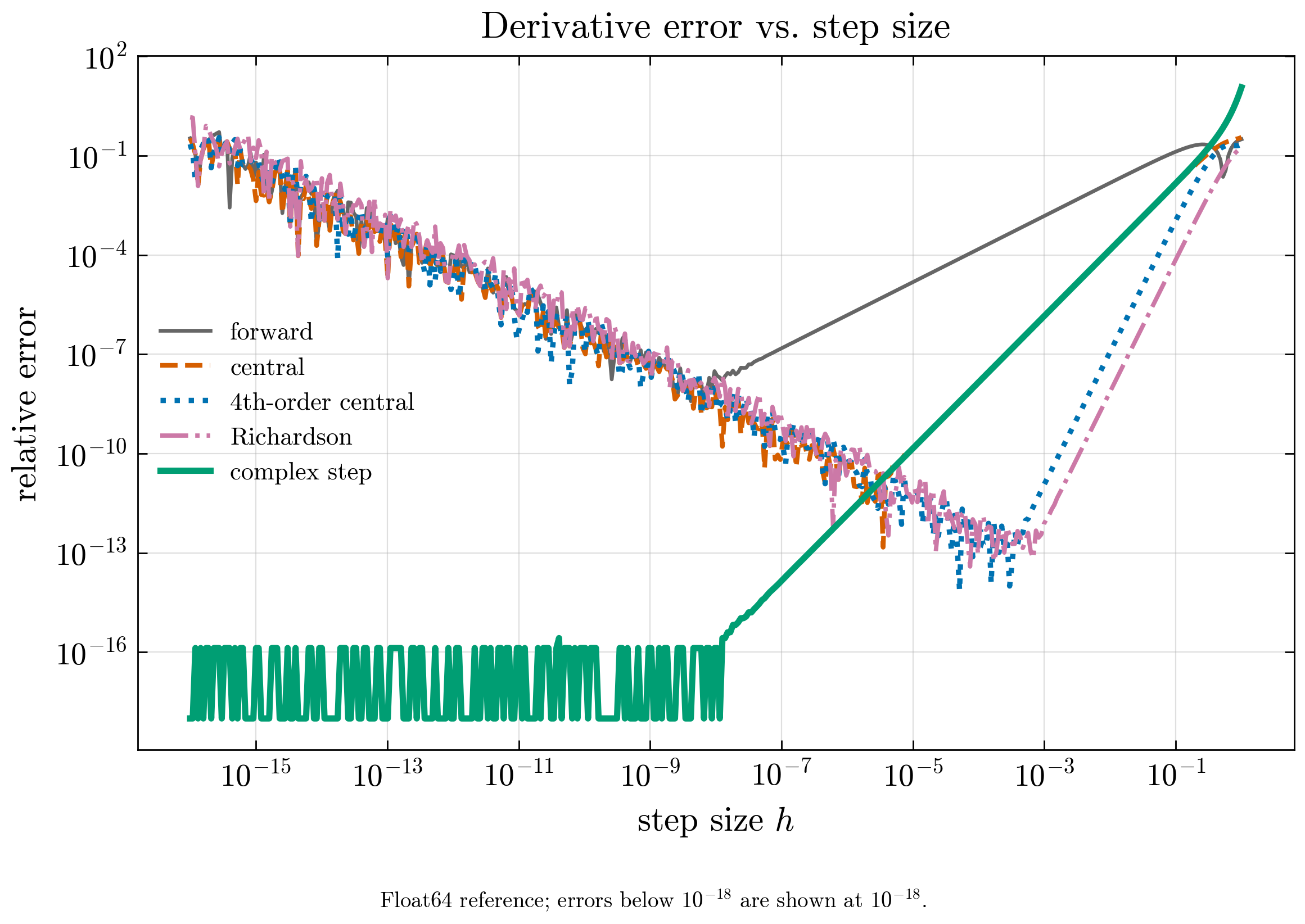
Relative derivative error versus step size for a smooth analytic function

Read from right to left as the step decreases. The finite-difference curves reach a minimum and then rise. The complex-step curve settles near floating-point precision over a broad range of small steps.

The distinction is clearest on the left side of the plot. Higher-order formulas shift the useful range of finite-difference steps, but their errors eventually grow too. Complex step has already reached an accuracy plateau and stays there. This makes it particularly convenient when we want an accurate first derivative without searching for a narrow optimal step.

How one `abs` can ruin it

There is a catch worth seeing before applying the trick to a large code.

Consider $g(x)=|x|$ at $x_0=0.5$ . The function is perfectly smooth in a neighborhood of that point, and $g'(x_0)=1$ . But Python's abs applied to a complex number returns its magnitude:

|x+ih|=\sqrt{x^2+h^2}.

That result is real. Its imaginary part is zero, and the complex-step estimate is zero for every nonzero $h$ :

def g(z):
    return abs(z)
 
h = 1e-30
print(g(0.5 + 1j * h).imag / h)  # 0.0; the derivative is 1.0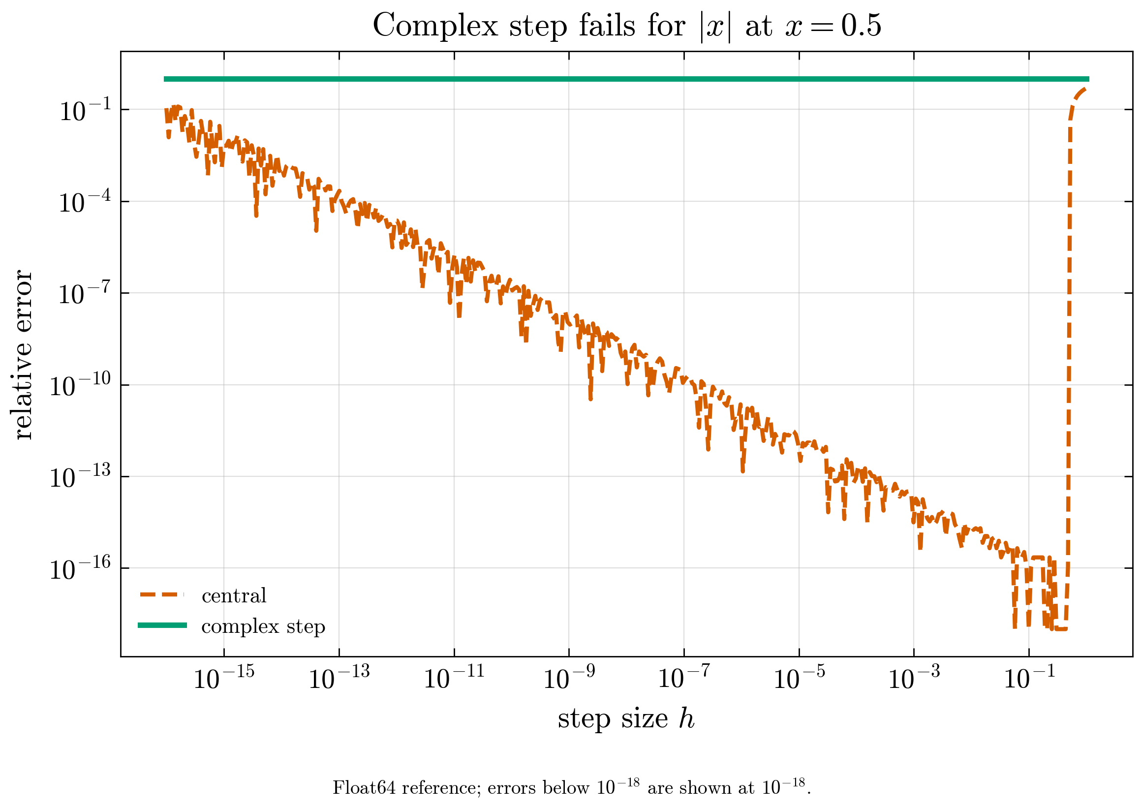

Failure of complex-step differentiation when the implementation uses complex magnitude

The solid green complex-step curve stays at a relative error of one: the estimate is zero, while the true derivative is one. Central differences give accurate estimates over a range of step sizes.

The problem here is the extension used by the code. Near a positive real point, $g(x)=x$ , whose analytic extension is simply $g(z)=z$ . Complex magnitude computes a different function of $z$ and does not satisfy the assumptions behind the formula.

Accepting complex inputs is not enough. Operations such as complex magnitude, conjugation, extracting .real, or casting to a real data type can invalidate the derivative even when the original real function is smooth.

Branches, min/max, thresholds, and event detection also need attention. A fixed smooth branch can sometimes be handled correctly, but a change of branch may introduce a point where the ordinary derivative does not exist. Finite differences remain useful when only real evaluations are available; they still need care near such points.

When the function is a simulation

Suppose a parameter $p$ controls the growth rate in the logistic equation:

\frac{dy}{dt}=py(1-y),\qquad y(0)=0.2.

Our output is the solution at $T=5$ , $J(p)=y(T;p)$ , and we evaluate its derivative at $p=1.2$ . The numerical solution uses fourth-order Runge–Kutta with 4,000 fixed time steps. To apply complex step, we give the solver $p+ih$ and compute

J'(p)\approx\frac{\operatorname{Im}J(p+ih)}{h}.

The imaginary perturbation now passes through every time step. The solver's state arrays and arithmetic must support complex values throughout.

This example has a closed-form solution, so we can check the numerical derivative independently:

y(T;p)=\frac{1}{1+Ae^{-pT}},\qquad A=\frac{1-y(0)}{y(0)}=4.

Differentiating that expression gives the reference used in the plot:

J'(p)=\frac{TAe^{-pT}}{(1+Ae^{-pT})^2}.

Relative error in the derivative of an ODE solution with respect to a parameter

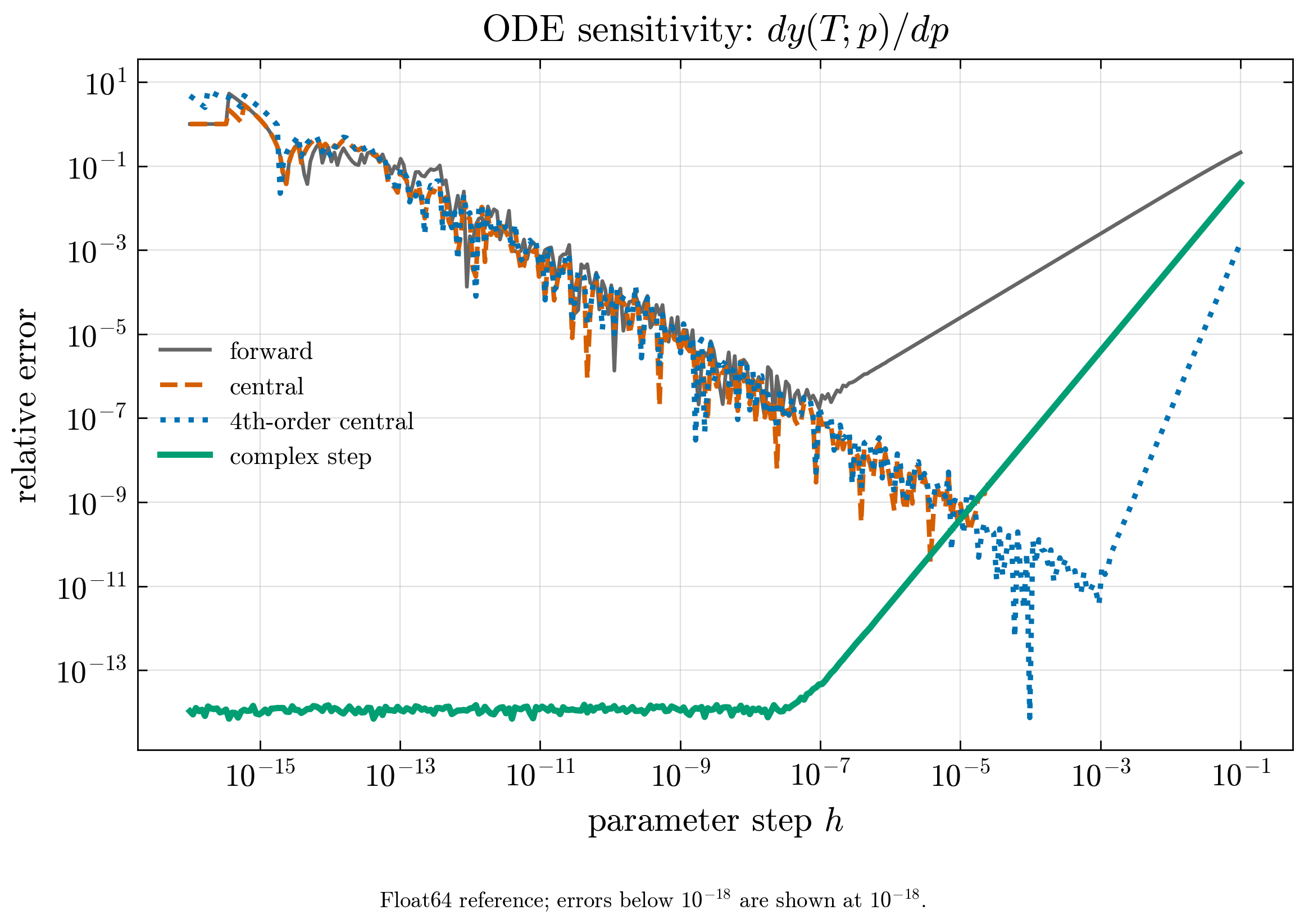
The ODE comparison shows a broad region of small steps where complex step remains accurate, while the finite-difference errors grow.

Complex step differentiates the implemented calculation. Agreement with its derivative does not guarantee agreement with the exact differential equation: time steps, solver tolerances, and other approximation errors still matter.

This distinction is useful in practice. First check whether the differentiation method behaves consistently for a fixed calculation. Then refine the solver to see whether the derivative converges to the quantity you actually want.

Even when the mathematics supports complex step, numerical routines can introduce imaginary rounding noise that overwhelms the derivative signal at tiny steps. The implementation must preserve the small imaginary response, not merely accept complex inputs.

What about second derivatives?

Everything above concerns first derivatives. For a second derivative, the natural extension is

f''(x)\approx\frac{2\left[f(x)-\operatorname{Re}f(x+ih)\right]}{h^2}.

But now the information we need sits in the real part, alongside $f(x)$ . Extracting it requires subtracting nearly equal numbers again: the small-step advantage is lost.

One way forward is to give the derivative another component to occupy. You may know quaternions as an extension of complex numbers. The multicomplex-step method uses a different algebra, with commuting imaginary units. Multicomplex numbers are defined recursively by

\mathbb{C}_0=\mathbb{R},\qquad \mathbb{C}_n=\{z_1+z_2 i_n:\ z_1,z_2\in\mathbb{C}_{n-1}\},

where $i_k^2=-1$ and $i_k i_\ell=i_\ell i_k$ . The first new case is a bicomplex number:

z=a+b i_1+c i_2+d i_1i_2,\qquad a,b,c,d\in\mathbb{R}.

For a suitable analytic function, the coefficient of $i_1i_2$ now carries the second derivative:

f''(x)=\frac{[f(x+h i_1+h i_2)]_{i_1i_2}}{h^2} +\mathcal{O}(h^2),

where $[\cdot]_{i_1i_2}$ means “take the coefficient of $i_1i_2$ .” No subtraction of the function value is needed. Additional commuting units extend the idea to higher derivatives; quaternion units do not obey the multiplication rules this construction needs.

The implementation is a separate challenge. Standard complex-number support is insufficient: arithmetic, elementary functions, and the solver must all handle multicomplex values. In practice, this may mean using or writing specialized libraries. The paper below develops the method; a working implementation deserves a post of its own.